CFD Simulations of Multiphase Flows: Interaction of Miscible Liquids with Different Temperatures

Abstract

The incorporation of new equations to extend the applicability of open-source computational fluid dynamics (CFD) software according to the user’s needs must be complemented with code verification and validation with a representative case. This paper presents the development and validation of an OpenFOAM^®-based solver suitable for simulating multiphase fluid flow considering three fluid phases with different densities and temperatures, i.e., two miscible liquids and air. A benchmark “dam-break” experiment was performed to validate the solver. Ten thermistors measured temperature variations in different locations of the experimental model and the temperature time series were compared against those of numerical probes in analogous locations. The accuracy of the temperature field assessment considered three different turbulence models: (a) zero-equation, (b) k-omega (Reynolds averaged simulation; RAS), and (c) large eddy simulation (LES). The simulations exhibit a maximum time-average relative and absolute errors of 9.3% and 3.1 K, respectively; thus, the validation tests proved to achieve an adequate performance of the numerical model. The solver developed can be applied in the modeling of thermal discharges into water bodies.

1. Introduction

Multiphase flow can be defined as a flux in which phases with different states of matter (e.g., solid, fluid, gaseous) or properties (e.g., temperature, density, viscosity) interact simultaneously within a system [1]. Since deriving exact analytical methods for evaluating multiphase flow is very complex [2], numerical methods for the solution of the governing equations are necessary. In this regard, computational fluid dynamics (CFD) techniques are widely used to study multiphase flows. These methods use computer-generated numerical solutions of the governing equations for fluid dynamics. Nevertheless, numerical schemes require calibration and validation to reduce the uncertainties when approaching real physics [3,4,5,6,7].

The need for improved and validated CFD numerical tools arises from the different engineering fields and applications concerning multiphase flow, such as submarine groundwater mixing processes [8,9,10], thermal discharge of ocean thermal energy conversion (OTEC) plants [11,12,13], nuclear thermal discharge [14,15,16], and mixing flows in a dam-break phenomenon [17].

The use of an open-source CFD framework allows the extension and modification of the native codes for the generation of additional models, not necessarily available in commercial CFD software [18]. Among the wide range of CFD tools available, OpenFOAM^® has gained popularity, mainly because of the cost reduction due to the elimination of license fees [19], the possibility of extending and modifying the native codes, and its high level of abstraction allowing the analysis of a variety of multiphase flow systems. Examples of code extension in OpenFOAM^® are the wave generation toolbox Waves2Foam [20] and the development and implementation of the direct and adjoint incompressible Navier-Stokes equations for the instability and sensitivity analysis of flows using OpenFOAM^® [21].

Several authors have investigated multiphase flows that involve free-surface flow with liquid-liquid interaction phenomena in OpenFOAM^®. For instance, in chemical engineering applications, Wardle [18] simulated the solvent extraction in centrifugal contractors, modeling a multiphase flow through the volume of fluid (VOF) methodology and considering turbulence effects with the large eddy simulation (LES) approach. Later, Wardle and Weller [22] proposed an OpenFOAM^®-based methodology to investigate the phase-segregated and dispersed flow regimes in stage-wise liquid-liquid extraction device flows. Lopes [23] investigated free-surface flows with air-entrainment with applications to hydraulic problems. Tripathi and Buwa [24] developed a model to simulate gas-liquid (i.e., two-phase) boiling flows. In their development, they included the k-ε turbulence model and energy transport accompanied by phase change and different inter-phase coupling forces, validating the applicability of the software with benchmark boiling experiments. A more recent contribution was presented by Nabil and Rattner [25], who proposed a solver to investigate liquid-vapor phase changes by simulating a two-phase flow with a thermally driven phase change.

To the best of the authors’ knowledge, a validated open-source solver which simulates the thermal equilibrium and mixing of two liquid phases under free-surface conditions is not yet available. Therefore, this paper presents the development and validation of an OpenFOAM^®-based solver suitable for simulating the thermal equilibrium and the mixing of two liquid-phases with a free-surface condition [26]. The solver presented can handle three fluid phases with different densities and temperatures, two of which are miscible liquid-phases, while the third one could represent a non-miscible gas-phase. The main contribution is the implementation of the energy equation in terms of the temperature field for the two miscible liquid-phases. Temperature spatiotemporal distribution within an experimental model of a multiphase dam-break validated the computed temperature field under different turbulence approaches.

2. Development of the CFD Model

The numerical model was coded as a new multiphase solver for OpenFOAM^®, which features: (i) a multiphase fluid flow consisting of three phases with different density and temperature, i.e., two of the phases are liquid and miscible, and the third is air; (ii) incompressibility in all phases; thus, the solver application is limited to low Mach number flows, i.e., $Ma<0.3$ [27]; (iii) phase changes are not allowed in the simulation, e.g., boiling and condensation; and (iv) constant diffusion coefficient and viscosity.

Following the solvers’ name convention in OpenFOAM^®, the solver implemented was named interMixingTemperatureFoam (IMTF), where “interMixing” stands for the ability to solve the interaction between 3 incompressible fluids, two of which are miscible, and “Temperature” stands for the implementation of the energy equation in terms of the temperature field. Turbulence models, mesh generation schemes, and other generic utilities are available as part of the OpenFOAM^® toolbox for case setting and running.

2.1. Governing Equations

The system of governing equations contains the mass conservation (Equation (1)), momentum conservation (Equation (2)), scalar quantities conservation (Equation (3)), volume fraction (Equation (4)) and energy conservation (Equation (5)) equations.

$$\nabla ·U=0$$

(1)

$$\frac{\partial \rho U}{\partial t}+\nabla ·\left(\rho UU\right)=\nabla ·\left(\mu \nabla U+\rho \tau \right)-\nabla p+\rho g+\sigma {\kappa }_{\alpha }\nabla \alpha$$

(2)

$$\frac{\partial \rho \varphi }{\partial t}+\nabla ·\left(\rho \varphi U\right)=\nabla ·\left(D\nabla \varphi \right)+q_{\varphi }$$

(3)

$$\frac{\partial \alpha }{\partial t}+\nabla ·\left(\alpha U\right)+\nabla ·\left(U_r\alpha \left(1-\alpha \right)\right)=0$$

(4)

$$\frac{\partial \rho c_{p}T}{\partial t}+\nabla ·\left(\rho c_{p}TU\right)=\nabla ·\left(k\nabla T\right)+q_{\varphi }$$

(5)

where $t$ is the time, $U$ the velocity vector, $\rho$ the fluid density, $\mu$ the dynamic viscosity, $p$ the pressure, $g$ the gravitational acceleration, $\varphi$ a scalar quantity, $D$ the diffusion coefficient, ${\kappa }_{\alpha }$ the surface curvature, $\sigma$ the surface tension, $\alpha$ a scalar field for the identification of the phases or phase volume fraction, $U_r$ the relative velocity, $c_p$ the specific heat capacity, $T$ the temperature, $k$ the thermal conductivity, and $q_{\varphi }$ is a source/sink term of $\varphi$.

The momentum equation is described by $\tau$ as the Reynolds stress tensor (Equation (6)), with ${\mu }_t$ being the dynamic eddy viscosity or turbulent viscosity, $S=\frac{1}{2}\left(\nabla U+{\left(\nabla U\right)}^T\right)$ the rate of deformation tensor, $k_t$ the turbulent kinetic energy per unit mass, and $I$ the Kronecker delta.

$$\tau =\frac{2}{\rho }{\mu }_{t}S-\frac{2}{3}{k}_{t}I$$

(6)

Equations (1) and (2) constitute the Reynolds averaged Navier-Stokes (RANS) equations, while the interphase between the non-miscible and miscible phases is obtained through the VOF method, as described by Hirt and Nichols [28].

To model the mixture between the liquid phases, Equation (3) includes the diffusion coefficient $D$ [m²s⁻¹] which is the proportionality constant of Fick’s law and represents the ease with which each solute moves in the solvent. The diffusion coefficient was considered to be constant over time for practical purposes.

The implementation of the energy conservation equation in terms of the temperature (Equation (5)) is required to model the temperature field. Because no phase changes are contemplated in the new solver, the source term $q_{\varphi }$ is null. The values of the Prandtl number and the specific heat capacity [J kg⁻¹ K⁻¹] are introduced as constant data for each of the three phases. The Prandtl number ($Pr$) is a dimensionless parameter that indicates the effectiveness of the conduction compared to the convection when transferring heat proportional to the ratio of momentum diffusivity to thermal diffusivity (i.e., the quotient of the viscous diffusion rate and the thermal diffusion rate). Specific heat capacity is an intensive property that describes the amount of energy (heat) required to increase the temperature of 1 kg of matter by 1 K. The thermal conductivity [J m⁻¹ s⁻¹ K⁻¹] is an intensive property that measures the heat conduction capacity of a substance (Equation (7)). To model the temperature field with the energy conservation equation, the thermal conductivity for the mixture is calculated through a weighted arithmetic mean. Therefore, $k$ is affected by the fraction phase in each cell, as shown in Equation (8).

$$k=\rho \upsilon \frac{c_p}{Pr}$$

(7)

$$k={\alpha }_1{\rho }_1{\upsilon }_1\frac{c_{p1}}{P{r}_1}+{\alpha }_2{\rho }_2{\upsilon }_2\frac{c_{p2}}{P{r}_2}+{\alpha }_3{\rho }_3{\upsilon }_3\frac{c_{p3}}{P{r}_3}$$

(8)

Specific heat capacity for the mixture $\rho \times c_p$, as well as the heat flux $\rho \times \phi \times c_p$, are obtained respectively as:

$$\rho \times c_p={\alpha }_1{\rho }_1{c}_{p1}+{\alpha }_2{\rho }_2{c}_{p2}+{\alpha }_3{\rho }_3{c}_{p3}$$

(9)

$$\rho \times \phi \times c_p={\alpha }_1\phi {\rho }_1{c}_{p1}+{\alpha }_2{\rho }_2\phi c_{p2}+{\alpha }_3{\rho }_3\phi c_{p3}$$

(10)

Equations (8)–(10) are associated with the Laplacian, the partial derivative, and the divergence of Equation (5), respectively.

2.2. Solver Coding

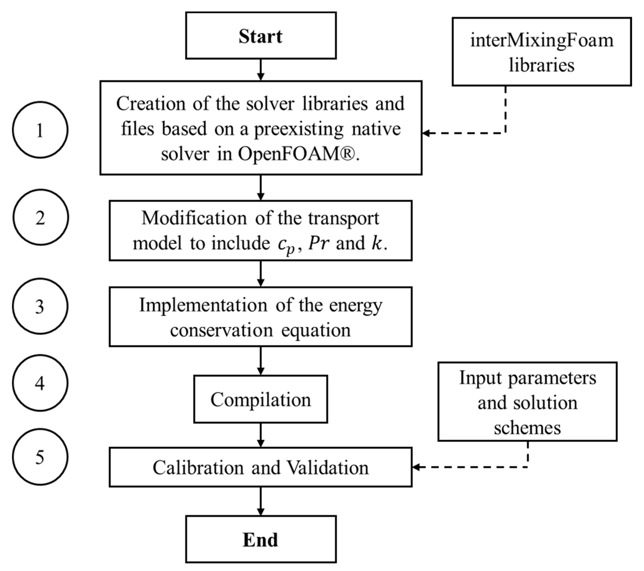
The algorithm of the IMTF solver can be summarized in five main steps as described below and outlined in the flow chart in Figure 1.

1

Creation of the solver libraries and files based on a preexisting native solver in OpenFOAM^®: The native solver interMixingFoam was used as a code base for the new IMTF solver; thus, they share the same directory tree and name conventions for the files. interMixingFoam allows the simulation of multiphase fluid flow considering two miscible phases. An extensive interMixingFoam solver error analysis in presented in [17].

2

Modification of the transport model: The three directories which contain the code for the transport model (as found in the native interMixingFoam) were modified to include the specific heat capacity $c_p$ and Prandtl number $Pr$ for each phase, as well as the estimation of the thermal conductivity for the mixture $k$.

3

Coding of the energy conservation equation: Equation (5) was programmed in an individual file.

4

Compilation: The new solver was compiled in the project directory.

5

Calibration and validation: This step includes the case setup, considering the parameters initially required for each of the three phases (i.e., density, kinematic viscosity, Prandtl number, specific heat capacity, and temperature) and the solution schemes, considering the new parameters for the energy equation. The turbulence model, the control properties, and other solution schemes are given analogously to any case in OpenFOAM^®.

The files for implementing IMTF in OpenFOAM^® version 4.0 are openly available as Supplementary Material in http://dx.doi.org/10.17632/kcjdyvjnfk.1.

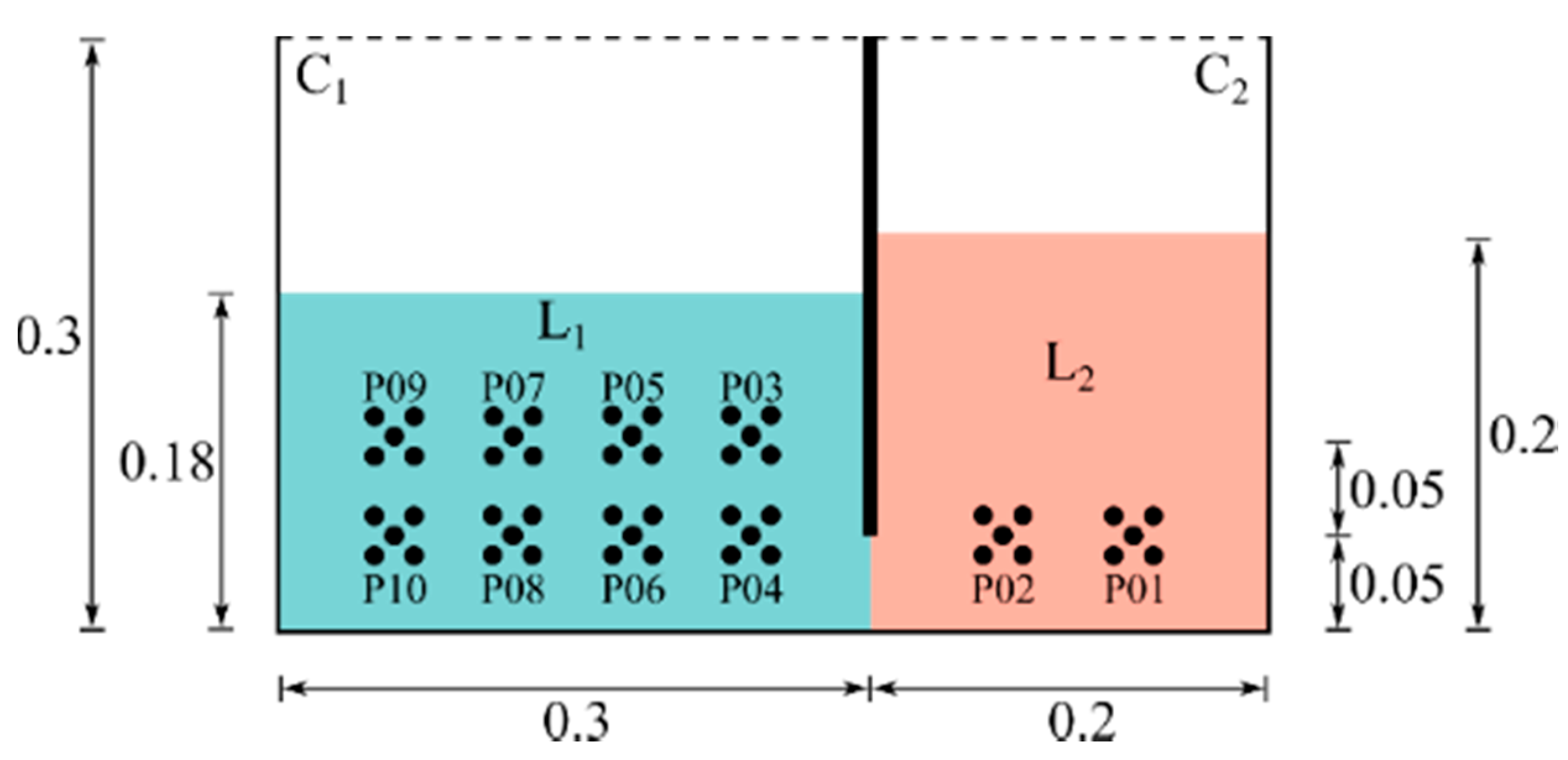
3. Experimental Setup

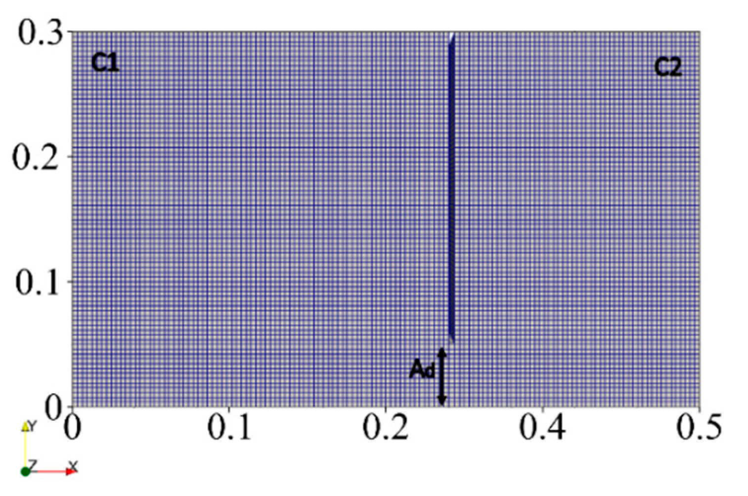
Laboratory benchmark tests of dam-break type were carried out to evaluate the validity of the IMTF solver. For this purpose, an acrylic container of $0.50 \mathrm{m}$ length,$0.30 \mathrm{m}$ height, and $0.10 \mathrm{m}$ depth was built (Figure 2a,b). The container was divided into two open compartments by a vertical gate (compartment C1, and compartment C2, Figure 2). The acrylic container was instrumented with ten LM35-thermistors (Texas Instruments, Dallas, TX, USA), with a response time of ~8 s. Thermistors S01 and S02 were located in C2, while S04, S06, S08, and S10 were placed in the bottom row in C1, and S03, S05, S07, and S09 in the top row in C1, as shown in Figure 2.

The acrylic container was instrumented with ten thermistors of type LM35 in TO-92 package, which are produced by Texas Instruments and are calibrated in degrees Celsius. They provide an ensured accuracy in the range of 25 °C to 50 °C of ±0.6 °C and low self-heating of 0.08 °C in still air. The thermal inertia of the LM35 in TO-92 package results in a reaction time of 8 s to reach 90% of the experienced temperature gradient [29].

Before the start of the experiments, each compartment was filled with water at different temperatures, and hence different densities (

Table 1. Depth, density, and temperature values of L1, L2, and air.

Property	L1	L2	Air
Depth (m)	0.18	0.20	-
Density (kg/m3)	1002	989	1
Temperature (K)	291.95	325.35	292.15

): C1 was partially filled with water (L1), and C2 with heated water (L2). The water density was measured with a hydrometer 151H ($0.001 \mathrm{kg}/{\mathrm{m}}^3$ resolution). The heated water was dyed with a color additive (at a low concentration to ensure that its influence on density was negligible) to contrast the two liquid phases and to monitor possible leakage before gate opening.

The tests began with the sudden lift of the gate from its initial condition ($t=0.0 \mathrm{s}$) until it reached a height of 0.05 m (see aperture distance, $A_d$, Figure 2). The lifting of the gate allowed multiphase flow mixing due to density and temperature gradients and pressure gradients caused by the different water levels in each compartment. The ten thermistors recorded the temperature of the liquids for 44 s with a frequency of 100 Hz.

4. Numerical Simulations

4.1. Numerical Setup

Temperature data were extracted from numerical probes placed at locations analogous to the thermistors. Since the thermistors occupy a certain surface ($~0.25{ \mathrm{cm}}^2$) instead of a punctual location in space, the mean value of five numerical probes within $0.25{ \mathrm{cm}}^2$ were used for the comparison, i.e., numerical probes yielded 10 probes sets (Figure 3). The order of probes sets P01 to P10 matches the order of thermistors S01 to S10 (Figure 2).

4.1.1. Constant Properties

Transport properties such as density and temperature were introduced according to the measured data. The value of the diffusion coefficient was taken from Holz et al. [30] for a temperature of 293.15 K, while surface tension, Prandtl number, specific heat capacity, and kinematic viscosity values correspond to the temperature of each fluid.

Table 2. Transport properties for the three fluid phases.

Phase Property	L1	L2	Air
Density (kg m−3)	1002	989	1
Kinematic viscosity (m2 s−1)	1.01 × 10−6	0.55 × 10−6	1.51 × 10−6
Temperature (K)	291.95	325.35	292.15
Prandtl number	6.62	3.42	0.71
Specific heat capacity (J kg−1 K−1)	4190	4182	1005
Surface tension (N m−1)	0.07	0.069	-
Diffusion coefficient (m2 s−1)	2.025 × 10−9		-

summarizes the input data of the numerical simulation for each phase.

The gravity acceleration was set to $9.81{ \mathrm{ms}}^{-2}$, acting in the negative direction of the vertical “Y” coordinate. For comparison purposes, three turbulence models were tested: (i) zero-equation turbulence; (ii) k-omega; and (iii) the LES model.

4.1.2. Boundary Conditions

InletOutlet and totalPressure boundary conditions were set at the top of the domain to simulate a free-surface condition. The front and back faces, which simulate the lateral walls of the container, were set with an empty boundary condition, i.e., two-dimensional simulation. Simple zeroGradient and empty boundary conditions were set to the density and temperature fields. The starting velocity field boundary conditions were set with a velocity equal to 0 m/s for all the fluid phases.

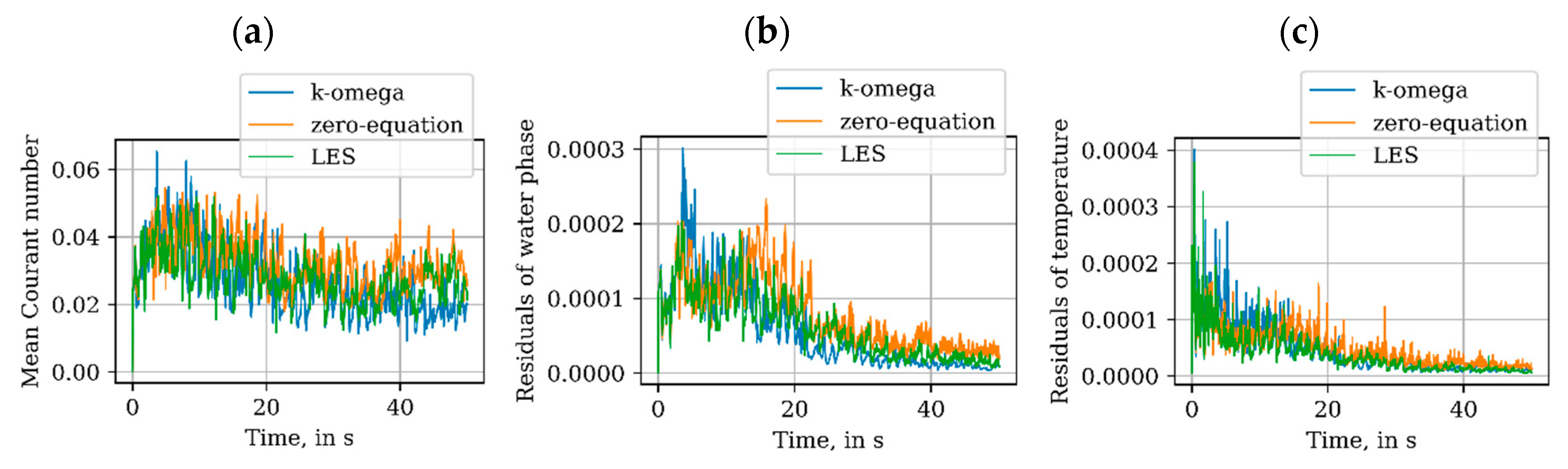
4.1.3. Control Settings and Solution Schemes

The simulation time was set to 43 s and results written every 0.001 s. The Courant number was defined considering the expression $Co=\frac{\delta t\left|U\right|}{\delta x}$, where $\delta t$ is the time step, which is 0.001 s for this case, and $\delta x$ is the cell size in the direction of the velocity $U$. A Courant number lower than 1.0 is required to ensure that fluid particles move (at most) from one cell to another within one-time stepA Courant number lower than 1.0 is required to ensure that fluid particles move (at most) from one cell to another within one-time step. Thus, to stabilize the solution, the maximal Courant number was set to 0.25 (Figure 4a), and the maximal time step to 0.01 s.

For coupling equations for momentum and mass conservation, the PIMPLE (merged PISO-SIMPLE) algorithm was used, which is a combination of the SIMPLE (semi-implicit method for pressure-linked equations) and PISO (pressure-implicit split-operator) algorithms. A generalized geometric-algebraic multi-grid (GAMG) solver was chosen for the pressure field, a smooth solver for the fluid phases and the velocity fields, as well as a preconditioner bi-conjugate gradient (PBiCG) for temperature.

Mean Courant number and residuals for water phase and temperature field were plotted to inspect the stability and convergence of the numerical solution considering the three turbulence models applied (Figure 4). The mean Courant number remained below 0.065, and residuals of both water phase and temperature tended to zero, which means that the discretized governing equations solution was balanced and convergence was achieved during the simulation.

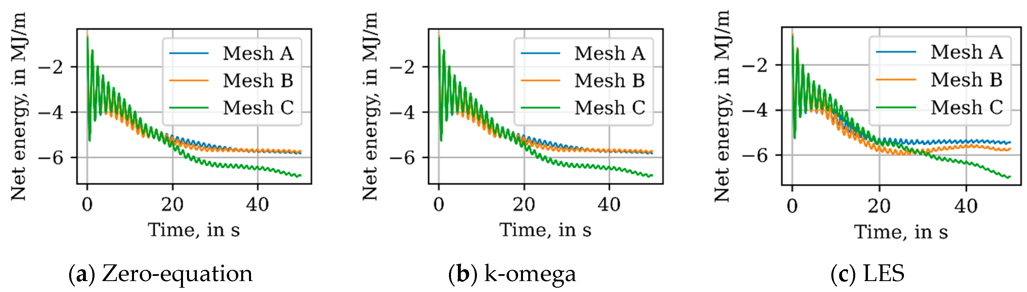
4.2. Mesh Sensitivity Analysis

Since discretization errors are one of the main sources of computational errors, a grid-space and time-step sensitivity analysis was performed. Three mesh configurations were tested: Mesh A, B and C (

Table 3. Characteristics of Mesh A, B, and C.

	Direction	Dimension (m)	Cell Number	Cell Size (cm)
Mesh A	X	0.50	196	0.2551
	Y	0.30	118	0.2542
	Z	0.10	1	0.10
Mesh B	X	0.50	139	0.3597
	Y	0.30	83	0.3614
	Z	0.10	1	0.10
Mesh C	X	0.50	98	0.5102
	Y	0.30	59	0.5085
	Z	0.10	1	0.10

). The refinement factor was set to $\sqrt{2}$ for both spatial and temporal discretization, i.e., second-order discretization schemes [6].

The mesh used in the numerical setup was discretized considering hexahedral cells in a Cartesian coordinate system. The X- and Y- directions were uniformly discretized so that the cell aspect ratio was ~1.0. The test case of the mesh convergence study was run for $t=50 \mathrm{s}$ and the results were printed each 0.1 s.

It was qualitatively observed that the three meshes produced similar results, but with small differences in eddy size and slight offsets in time due to the fast speed of the fluid motion of a dam-break case. To study the mesh sensitivity, the heat flow through the aperture distance ($A_d$) was estimated by the product of density, velocity, temperature, and specific heat capacity. Then, the heat flux was integrated with respect to time.

Figure 5 shows the net energy for the three meshes as a function of time, for each turbulence model. As the mesh becomes finer, the results tend to show no difference between them; therefore, mesh independency is achieved. Results from Mesh A and B are very similar; however, computational costs are significantly higher for Mesh A.

Running time for Mesh A is ~61% higher than Mesh B, which is in turn ~27% higher than Mesh C. Considering the previous results and the running time optimization, Mesh B was selected to simulate the experimental test case (Figure 6).

5. Results and Discussion

5.1. Experimental Results

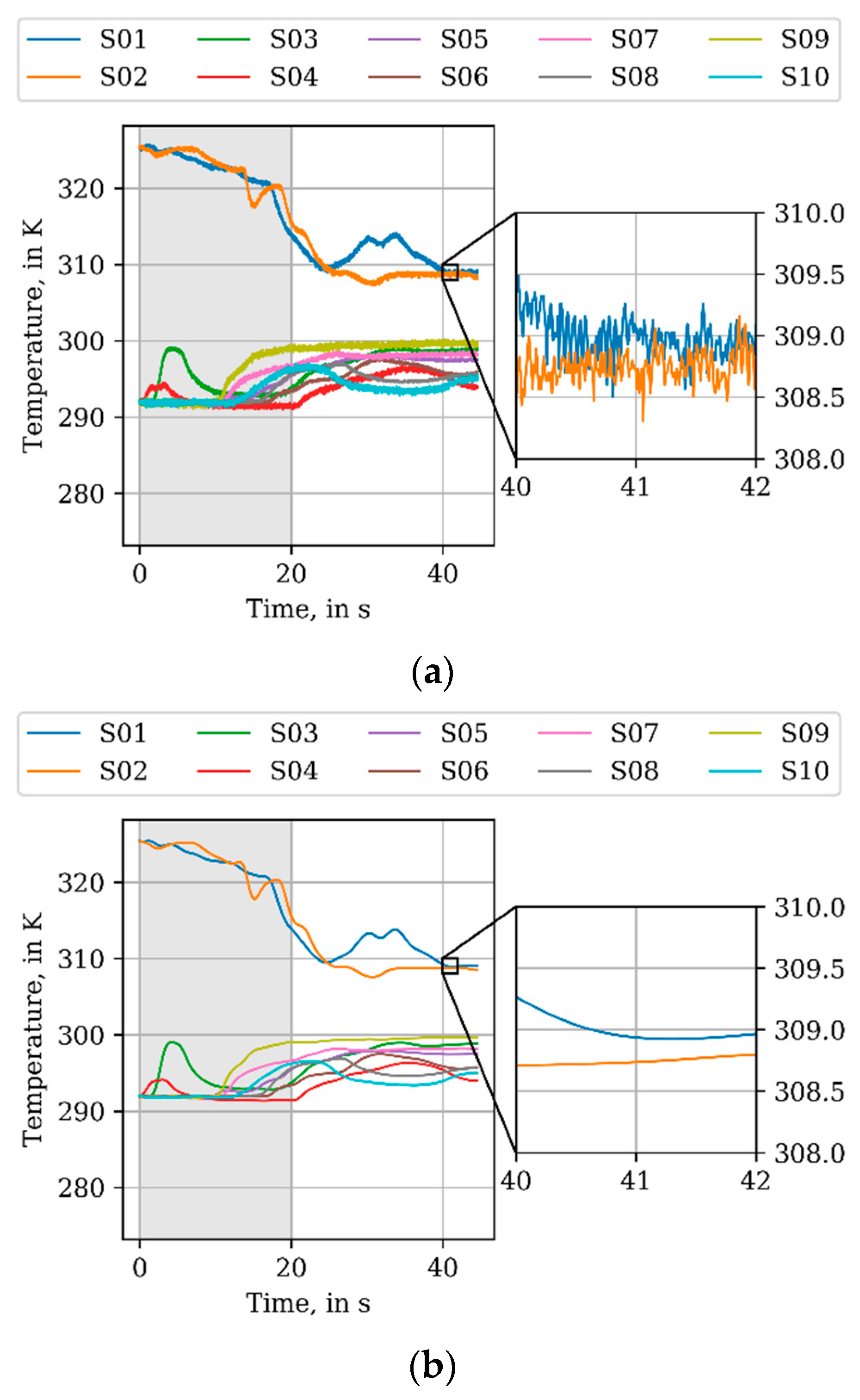
Figure 7 shows the data obtained by the thermistors during the experiments before (raw data) and after applying the Python 3rd order SciPy Butterworth low-pass filter to smooth the noise of the signal (https://www.scipy.org).

In Figure 7, the registered temperature at time zero corresponds to the temperature of L2 (heated water) for thermistors S01 and S02, and the temperature of L1 for S03 to S10. After the gate lifting at time zero, the temperature varies as L1 and L2 interact due to the difference of depths and temperatures. It was observed that in the first 20 s of the experiments the formation of eddies predominated. Nevertheless, these rapid fluctuations of temperature were not captured by the thermistors, since the response time was ~8 s. After 20 s, the flow tends to stabilize, the temperature gradient governs the fluid motion and gradually becomes time-independent (i.e., thermal equilibrium). Since the mixing was not complete, S01 and S02 maintain a higher temperature than the rest of the thermistors. Furthermore, the thermistors in the bottom row of C1 measured lower temperatures through time than those in the top row. Thus, there is a stratification of the temperature, which was visually corroborated in the experiments by means of the color contrast.

5.2. Numerical Results

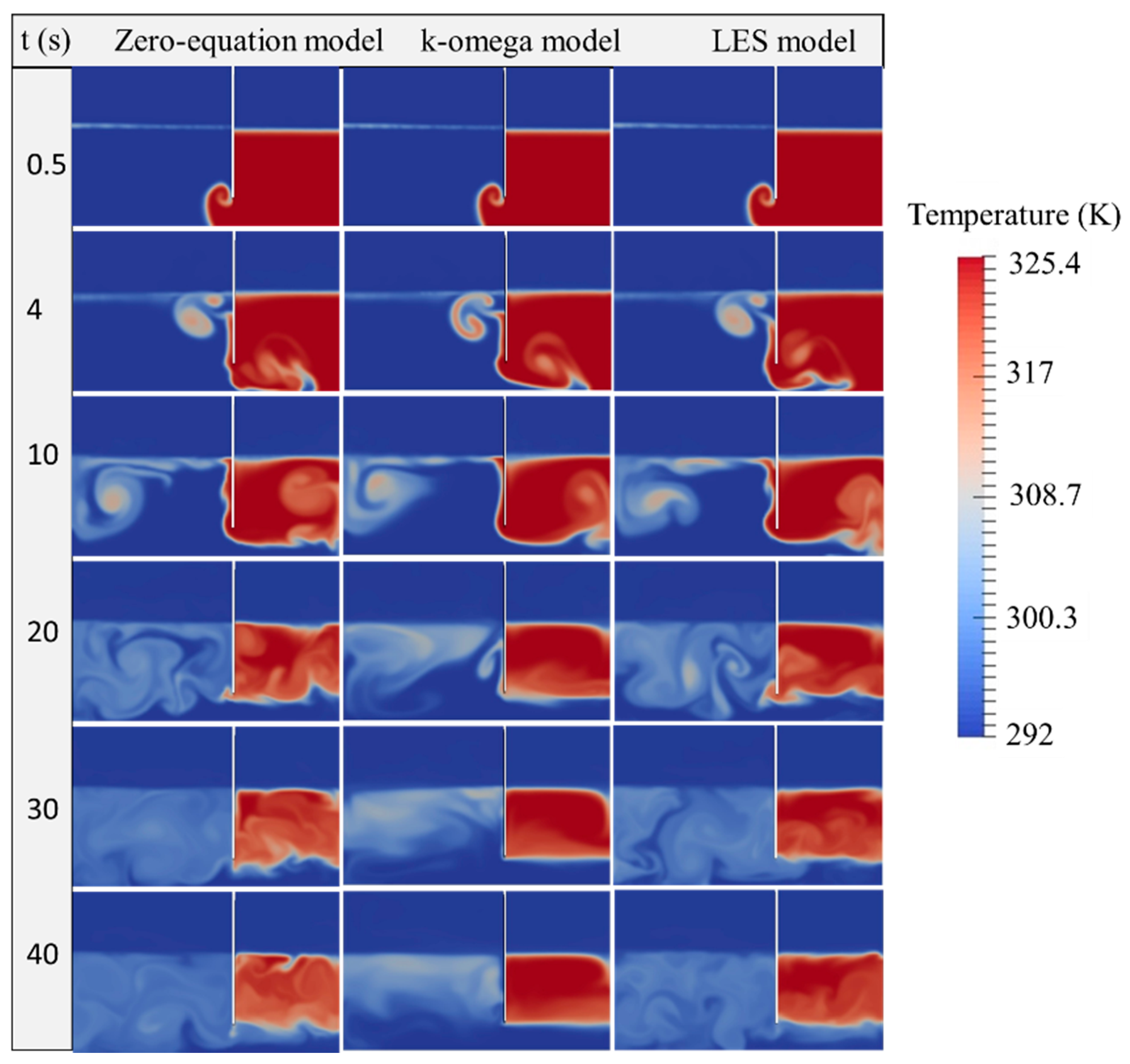
Figure 8 shows a qualitative comparison of specific time instants (0.5, 4, 10, 20, 30, and 40 s) between the three turbulence models tested. The turbulence model affects these results since it influences the mixing process, which is dominated by the speed of the dam-break and the formation of eddies during the transient phase of the experiments.

Figure 8 shows that at time $t=0.5 \mathrm{s}$ heated water from C2 started flowing to C1 due to the difference in water level between the compartments. A small eddy ($~5 \mathrm{cm}$) was formed on the right side of the aperture. There was no noticeable difference between the models at this point. At time $t=4 \mathrm{s}$ cold water from C1 entered C2 and there were some noticeable differences in the shapes and definition of eddies. At time $t=10 \mathrm{s}$ a cold-water layer was clearly displayed at the bottom of the container and the differences in eddies and temperature diffusion were clearer between the models. At time $t=20 \mathrm{s}$ the temperature in zero-equation was affected due to the presence of smaller eddies than those in the other two turbulence models. Thereafter (time $t=30 \mathrm{s}$ and $t=40 \mathrm{s}$) the flow tended to stabilize. In C2, the temperature in the upper layer remained higher than in the rest of the domain. The main difference between the turbulence models is that the temperature was more homogeneous in the zero-equation and LES models than in the k-omega model. Overall, in the first 20 s of the experiment large eddies were formed, and the temperature drastically fluctuated in time and space. After 20 s the mixture was more uniform for the zero-equation and LES models, and the stratification of the temperature field was more notable for the k-omega model.

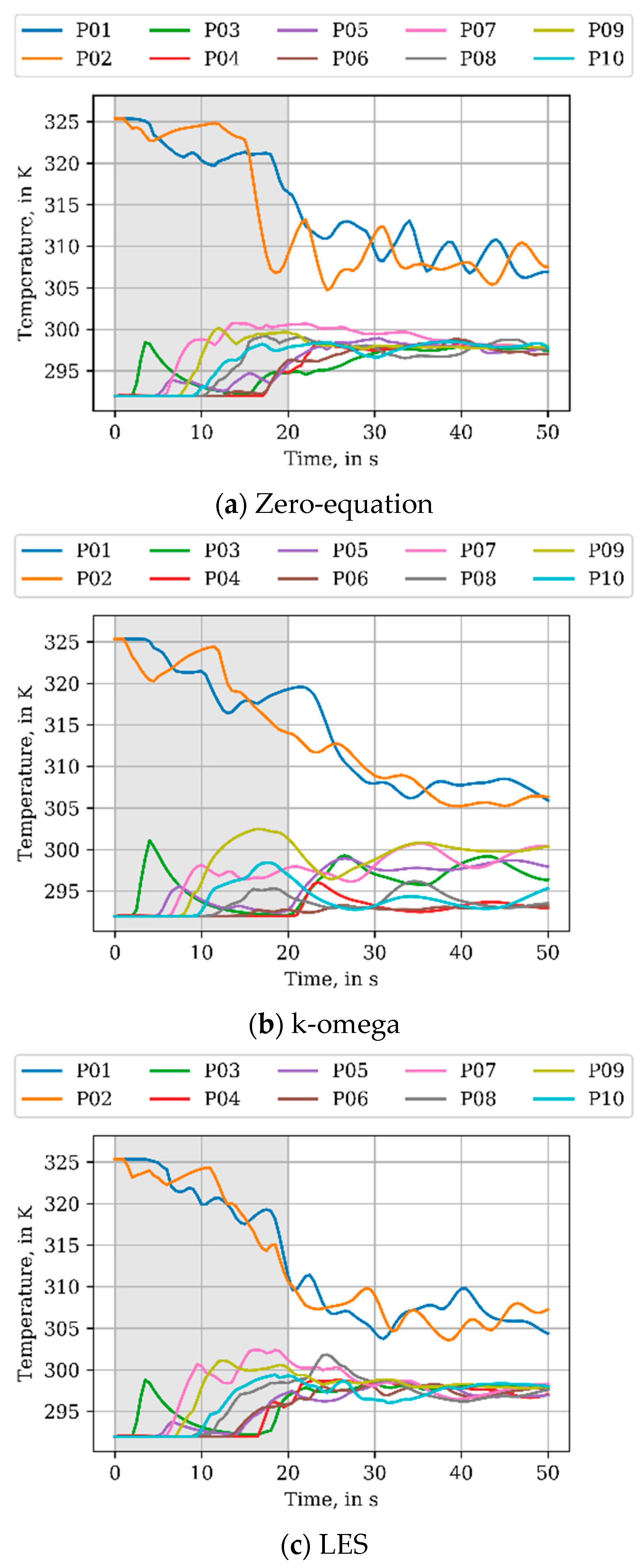
For each turbulence model, the temperature was recorded with a frequency of 10 Hz at the ten sets of numerical probes (P01 to P10 in Figure 3). To consider the response time of the thermistors, the temperature series were processed with Equation (11).

$$T_{i+1}=T_i-\lambda \left(T_i-T_{i+1}\right)$$

(11)

Equation (11) is affected by an inertia factor $\lambda$, which depends on the response time of the thermistors. For a response time of 8 s and reaching 90% of the temperature value, $\lambda =0.134$. Figure 9 shows the resulting temperature time series for the three turbulence models.

Figure 9 shows fluctuations of temperature in the first 20 s. Thereafter, the temperature tends to stabilize. The two probes in C2 (P01 and P02), registered higher temperatures than the probes in C1 (P03 to P10); showing that the mixing was not complete. The results in Figure 9 also reflect the uniformity of the mixing for the zero-equation and LES models, which was higher than that of the k-omega model.

5.3. Data Comparison

5.3.1. Absolute Error

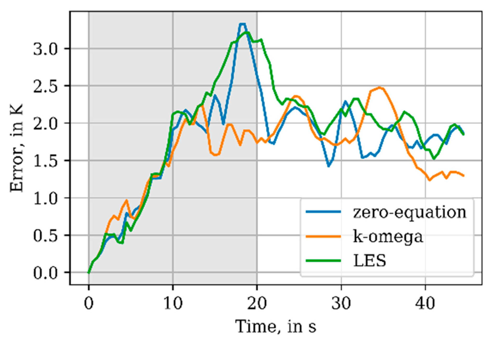
The absolute value of the difference between the measured temperatures and the temperatures given by the analogous numerical probes was obtained. Time-averaged absolute errors and spatial mean absolute errors show the distance between the observed and calculated values and their variability in time and space, respectively. Spatial mean absolute errors were obtained by averaging the absolute errors of the ten probe sets for each time step (Figure 10).

It can be seen in Figure 10 that the spatial mean absolute error first tended to increase, between 0 and 20 s, then it stabilized. The k-omega model gives the best results in terms of the spatial mean absolute errors. The LES and zero-equation models are more accurate, as the fluid flow stabilizes with time, but they have error peaks between 15 and 25 s.

Table 4. Time-averaged absolute errors, standard deviations, and root-mean-square errors (RMSE), in K.

	Zero-Equation Model			k-Omega Model			LES Model
Probe Set	Time-Averaged Absolute Error	SD	RMSE	Time-Averaged Absolute Error	SD	RMSE	Time-Averaged Absolute Error	SD	RMSE
P01	1.67	1.18	2.05	3.09	2.34	3.87	2.68	2.36	3.57
P02	2.47	2.76	3.70	2.13	1.38	2.54	2.48	1.67	2.99
P03	0.91	0.47	1.02	1.01	0.87	1.33	0.81	0.70	1.07
P04	2.12	1.44	2.56	1.38	1.17	1.81	2.40	1.73	2.96
P05	0.73	0.56	0.92	0.91	0.96	1.32	0.62	0.56	0.83
P06	1.04	0.94	1.40	1.75	1.64	2.40	1.17	1.03	1.56
P07	2.40	2.16	3.23	1.47	1.51	2.11	2.56	2.49	3.58
P08	2.01	1.58	2.56	1.39	1.20	1.84	2.27	1.70	2.84
P09	1.47	1.21	1.91	1.63	1.57	2.26	1.55	1.53	2.18
P10	2.57	1.61	3.03	1.38	1.21	1.84	2.54	1.53	2.96
P01 to P10	1.74	1.67	2.41	1.62	1.56	2.24	1.91	1.81	2.63

shows the time-averaged absolute errors, their standard deviation (SD), and the root-mean-square errors (RMSE) for each probe set. The last row in Table 4 presents the averaged absolute error in time and space, the SD, and the RMSE for each turbulence model.

The k-omega model gave the lowest averaged absolute errors, while the LES model gave the highest. The SD was also highest for the LES model, meaning a greater dispersion of the error data; while the k-omega model showed low dispersion for most of the probes. Meanwhile, the zero-equation model showed intermediate values for the averaged absolute errors, SD, and RMSE. Regarding the RMSE, the zero-equation and k-omega models were better at predicting observed data than the LES model. From this analysis, and considering the spatial mean absolute errors in Figure 10, the k-omega model is the most accurate model, followed by the zero-equation and LES models.

5.3.2. Relative Error

Each thermistor signal was compared with the signals of the ten sets of numerical probes through the relative error $E_i$, estimated for each turbulence model as:

$$E_i=\frac{\left|T_E-T_M\right|}{\Delta T}\times 100$$

(12)

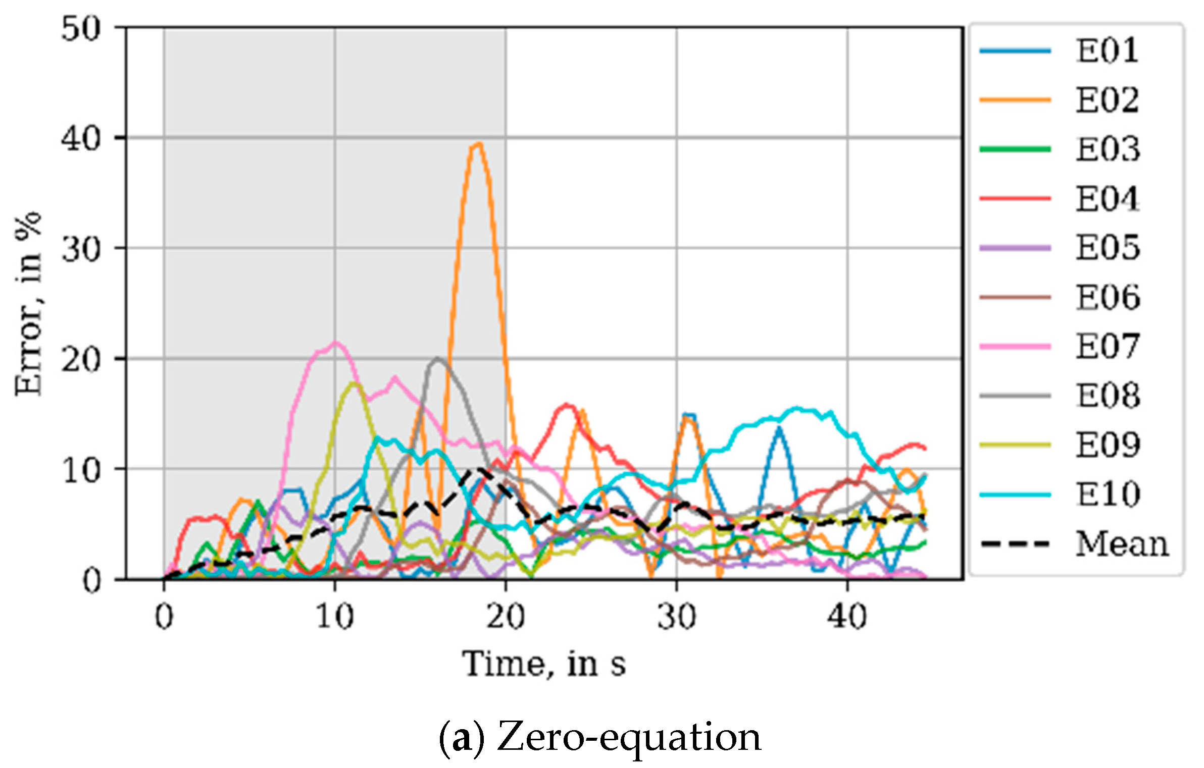
where $T_E$ and $T_M$, both in K, are the temperatures in the experiments and in the numerical simulation, respectively, and $\Delta T$ is the temperature difference between the two phases in time zero ($\Delta T_{t=0 s}=33.4 \mathrm{K}$). Figure 11 presents the time series of relative error for each of the ten probes sets, and the mean relative error, for the zero-equation, k-omega, and LES turbulence models, respectively. E01 to E10 are the relative error series for the corresponding numerical probe.

In Figure 11a, the zero-equation model shows sharp peaks for P02, P07, P09, and P01; nevertheless, the spatial mean errors remain below 10%. These errors could be attributed to the fluid flow stabilization time in the zero-equation model. It has previously been seen that zero-equation models tend to underestimate the energy dissipation compared to RAS and LES turbulence models [17]. Figure 11c also shows sharp error peaks in P01, P07, and P09, particularly. The results in Figure 11a,c, contrast with the results of Figure 11b, whose relative errors show lower peaks and, for most of the locations, they remain relatively stable and below 10%.

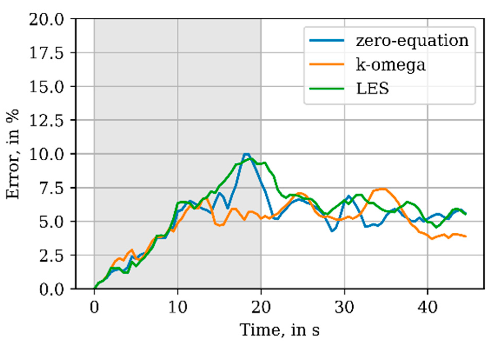
Figure 12 compares the time series of the spatial mean relative errors. The LES and zero-equation models give the highest errors, whereas the k-omega model presents the lowest spatial mean relative error through time.

The time-averaged relative error for each probe set is shown in

Table 5. Time-averaged relative error, in %, and its SD of the ten probe sets.

	Zero-Equation Model		k-Omega Model		LES Model
Probe Set	Relative Error	SD	Relative Error	SD	Relative Error	SD
P01	5.00	3.53	9.25	7.00	8.01	7.06
P02	7.38	8.26	6.39	4.13	7.43	5.00
P03	2.71	1.41	3.02	2.61	2.44	2.10
P04	6.34	4.31	4.13	3.52	7.20	5.18
P05	2.19	1.68	2.74	2.86	1.85	1.67
P06	3.11	2.81	5.25	4.90	3.50	3.09
P07	7.20	6.46	4.39	4.53	7.67	7.46
P08	6.02	4.72	4.17	3.58	6.81	5.08
P09	4.41	3.62	4.89	4.69	4.65	4.58
P10	7.69	4.82	4.13	3.63	7.60	4.57
P01 to P10	5.21	5.00	4.84	4.66	5.71	5.41

. The k-omega turbulence model has the highest time-averaged relative error for probe locations P01, P03, P05, P06, and P09; nevertheless, in P02, P04, P07, P08, and P10 it has the lowest error of the three models.

As with the averaged absolute errors, even though the k-omega model has the highest relative error in some probe locations, it has the lowest mean relative errors. The comparatively large errors in some of the probe locations for the zero-equation and LES models impact the SD values, which are higher than the k-omega model values.

Possible causes of discrepancy between the experimental results and the numerical simulation could be attributed to:

• The presence of a gate that must be lifted rapidly, rather than the ideal dam-break case, where there is no gate, but simply a membrane that instantly “disappears” [31].
• To install the gate, two rails were placed to guide the upward displacement of the gate, designed to interfere with the fluid motion as little as possible.
• The installation of the thermistors interfered with the fluid motions; however, they were adapted so that the wall in contact with the fluid was as smooth as possible, by perforating the front wall of the acrylic container.
• The heat induced by the thermistors was not considered during data processing; however, the electrical load was chosen to influence their operation as little as possible.
• The precision when filling the two compartments of the container and the measurement of the temperature and density; it was observed that small variations in the water level caused great differences in fluid flow behavior.
• Temperature-dependent parameters such as Prandtl number, specific heat capacity, kinematic viscosity, surface tension, and diffusion were assumed to be constant.
• The numerical domain is adiabatic beyond its boundaries, while the experimental model interacts with its environment.

Regardless of the above, the validation tests show acceptable errors of the numerical predictor for engineering purposes.

6. Conclusions

A new OpenFOAM^®-based solver was developed for simulating multiphase fluid flow, consisting of two-miscible liquid phases with different temperatures and densities in a free-surface condition. The IMTF solver was developed by programming the energy equation in terms of the temperature field on the preexisting OpenFOAM^® interMixingFoam native solver. To estimate the accuracy of the new solver, a wet dam-break experiment was designed and built, considering two compartments for miscible liquids with different temperatures (densities).

The experimental model was simulated with the solver developed, and both results were compared through error analyses with three different turbulence models: zero-equation, two-equation k-omega, and LES. Regardless of the differences between the turbulence models, none of them exhibited a time-averaged relative error of more than 9.3%. Furthermore, the spatial mean relative errors remained lower than 10%. On the other hand, the absolute errors were below 3.1 K for the time average values and 3.5 K for the spatial mean values.

The thermal inertia of the thermistors (i.e., response time) did not allow the capture of sudden temperature variations during the transient phase of the validation experiments. Further research with more precise instrumentation could help to validate the transient phenomena and to apply the solver developed in cases where this is relevant.

The solver described here could be applied in the simulation of thermal discharges, or in any system that involves multiphase flows, or miscibility of two liquid phases with different temperature/density.

Finally, the solver presented in this paper is subject to further improvement and testing by the CFD community and OpenFOAM^® developers, such as: the variation due to temperature of Prandtl number, specific heat capacity, kinematic viscosity, surface tension, and diffusion; the incorporation of a heat source term; and the ability to solve changes of state of matter. Further studies would be necessary when choosing the most adequate turbulence model in applications with a larger spatial domain and longer simulation times than those used for this study.

References

- Bello, O.O.; Falcone, G.; Teodoriu, C. Experimental validation of multiphase flow models and testing of multiphase flow meters: A critical review of flow loops worldwide. WIT Trans. Eng. Sci. 2007, 56, 97–111. [Google Scholar] [CrossRef] [Green Version]
- Kolev, N.I. Multiphase Flow Dynamics 1—Fundamentals, 4th ed.; Springer: Herzogenaurach, Germany, 2011; ISBN 978-3-319-15295-0. [Google Scholar]
- Eça, L.; Hoekstra, M. Code Verification of unsteady flow solvers with method of manufactured solutions. Int. J. Offshore Polar Eng. 2008, 18, 120–126. [Google Scholar]
- Eça, L.; Vaz, G.; Koop, A.; Pereira, F.; Abreu, H. Validation: What, Why and How. In Proceedings of the Proceedings of the ASME 2016 35th International Conference on Ocean, Offshore and Arctic Engineering, Busan, Korea, 19–24 June 2016. [Google Scholar]
- ITTC Resistance Committee. Uncertainty Analysis in CFD Verification and Validation Methodology and Procedures; ITTC: Fukuoka, Japan, 2008. [Google Scholar]
- Stern, F.; Wilson, R.V.; Coleman, H.W.; Paterson, E.G. Comprehensive Approach to Verification and Validation of CFD Simulations—Part 1: Methodology and Procedures. J. Fluids Eng. 2001, 123, 793–802. [Google Scholar] [CrossRef]
- Stern, F.; Wilson, R.; Shao, J. Quantitative V&V of CFD simulations and certification of CFD codes. Int. J. Numer. Methods Fluids 2006, 50, 1335–1355. [Google Scholar] [CrossRef]
- McCoy, C.A.; Corbett, D.R. Review of submarine groundwater discharge (SGD) in coastal zones of the Southeast and Gulf Coast regions of the United States with management implications. J. Environ. Manag. 2009, 90, 644–651. [Google Scholar] [CrossRef]
- Ma, Q.; Li, H.; Wang, X.; Wang, C.; Wan, L.; Wang, X.; Jiang, X. Estimation of seawater–groundwater exchange rate: Case study in a tidal flat with a large-scale seepage face (Laizhou Bay, China). Hydrogeol. J. 2014, 23, 265–275. [Google Scholar] [CrossRef]
- Luijendijk, E.; Gleeson, T.; Moosdorf, N. Fresh groundwater discharge insignificant for the world’s oceans but important for coastal ecosystems. Nat. Commun. 2020, 11, 1–12. [Google Scholar] [CrossRef] [Green Version]
- Kim, J.; Kim, H.-J. Numerical Modeling of Thermal Discharges in Coastal Waters. In Proceedings of the International Conference on Hydroinformatics; CUNY Academic Works, New York, NY, USA, 17–21 August 2014. [Google Scholar]
- Lee, H.; Kim, H.; Lee, S. Performance Characteristics of 20Kw Ocean Thermal Energy Conversion Pilot Plant. In Proceedings of the ASME 2015 9th International Conference on Energy Sustainability, San Diego, CA, USA, 28 June–2 July 2015; pp. 1–7. [Google Scholar]
- Wang, Z.; Tabeta, S. Numerical simulations of ecosystem change due to discharged water from ocean thermal energy conversion plant. In Proceedings of the OCEANS 2017-Aberdeen, Aberdeen, UK, 19–22 June 2017; IEEE: Piscataway, NJ, USA, 2017; pp. 1–5. [Google Scholar]
- Issakhov, A. Mathematical modeling of the hot water discharge effect on the aquatic environment of the thermal power plant by using two water discharge pipes. Int. J. Energy Clean Environ. 2018, 19, 93–103. [Google Scholar] [CrossRef]
- Thai, T.H.; Tri, D.Q. Modeling the Effect of Thermal Diffusion Process from Nuclear Power Plants in Vietnam. Energy Power Eng. 2017, 9, 403–418. [Google Scholar] [CrossRef] [Green Version]
- Issakhov, A.; Zhandaulet, Y. Numerical simulation of thermal pollution zones’ formations in the water environment from the activities of the power plant. Eng. Appl. Comput. Fluid Mech. 2019, 13, 279–299. [Google Scholar] [CrossRef] [Green Version]
- Rodríguez-Ocampo, P.E.; Ring, M.; Hernández-Fontes, J.V.; Alcérreca-Huerta, J.C.; Mendoza, E.; Gallegos-Diez-Barroso, G.; Silva, R. A 2D Image-Based Approach for CFD Validation of Liquid Mixing in a Free-Surface Condition. J. Appl. Fluid Mech. 2020. [Google Scholar] [CrossRef]
- Wardle, K.E. Open-Source CFD Simulations of Liquid–Liquid Flow in the Annular Centrifugal Contactor. Sep. Sci. Technol. 2011, 46, 2409–2417. [Google Scholar] [CrossRef]
- Tomislav, M.; Höpken, J.; Mooney, K. The OpenFOAM Technology Primer, 1st ed.; Sourceflux: Duisburg, Germany, 2014; ISBN 978-3-00-046757-8. [Google Scholar]
- Jacobsen, N.G.; Fuhrman, D.R.; Fredsøe, J. A wave generation toolbox for the open-source CFD library: OpenFoam. Int. J. Numer. Methods Fluids 2012, 70, 1073–1088. [Google Scholar] [CrossRef]
- Liu, Q.; Gómez, F.; Pérez, J.M.; Theofilis, V. Instability and sensitivity analysis of flows using OpenFOAM®. Chin. J. Aeronaut. 2016, 29, 316–325. [Google Scholar] [CrossRef] [Green Version]
- Wardle, K.E.; Weller, H.G. Hybrid multiphase CFD solver for coupled dispersed/segregated flows in liquid-liquid extraction. Int. J. Chem. Eng. 2013, 2013. [Google Scholar] [CrossRef]
- Lopes, P. Free-surface Flow Interface and Air- Entrainment Modelling Using OpenFOAM. Ph.D. Thesis, University of Coimbra, Coimbra, Portugal, 2016. [Google Scholar]
- Tripathi, R.G.; Buwa, V.V. Numerical Simulations of Gas-Liquid Boiling Flows Using OpenFOAM. Procedia IUTAM 2015, 15, 178–185. [Google Scholar] [CrossRef] [Green Version]
- Nabil, M.; Rattner, A.S. interThermalPhaseChangeFoam—A framework for two-phase flow simulations with thermally driven phase change. SoftwareX 2016, 5, 216–226. [Google Scholar] [CrossRef] [Green Version]
- Rodríguez-Ocampo, P.E. Modelación Termodinámica de Fluidos Multifásicos: Aplicación en Dispositivos de Conversión de Energía Térmica Oceánica; UNAM: Mexico City, Mexico, 2020. [Google Scholar]
- Remacle, J.; Lambrechts, J.; Seny, B. Blossom-Quad: A non-uniform quadrilateral mesh generator using a minimum-cost perfect-matching algorithm. International 2012, 89, 1102–1119. [Google Scholar] [CrossRef] [Green Version]
- Hirt, C.W.; Nichols, B.D. Volume of fluid (VOF) method for the dynamics of free boundaries. J. Comput. Phys. 1981, 39, 201–225. [Google Scholar] [CrossRef]
- Texas Instruments LM35 Precision Centigrade Temperature Sensors, SNIS159H Datasheet, 1999 [Revised Dec 2017]. Available online: https://www.ti.com/lit/ds/symlink/lm35.pdf (accessed on 14 September 2020).
- Holz, M.; Heil, S.R.; Sacco, A. Temperature-dependent self-diffusion coefficients of water and six selected molecular liquids for calibration in accurate 1H NMR PFG measurements. Phys. Chem. Chem. Phys. 2000, 2, 4740–4742. [Google Scholar] [CrossRef]
- Sanchez-Mondragon, J.; Hernández-Fontes, J.V.; Vázquez-Hernández, A.O.; Esperança, P.T.T. Wet dam-break simulation using the SPS-LES turbulent contribution on the WCMPS method to evaluate green water events. Comput. Part. Mech. 2019, 1–20. [Google Scholar] [CrossRef]
Figure 1.
Flow chart of the interMixingTemperatureFoam (IMTF) solver development for OpenFOAM®.
Figure 2.
(a) Experimental installation and (b) scheme of the experimental setup.
Figure 3.
Distribution of the numerical probe sets.
Figure 4.
Time series of the (a) mean Courant number, (b) water phase, and (c) temperature residuals.
Figure 5.
Time series of the net energy through Ad for the three mesh configurations and for the turbulence models: (a) zero-equation, (b) k-omega, and (c) large eddy simulation (LES).
Figure 6.
Numerical domain and mesh of the validation case.
Figure 7.
Temperature signal (a) before and (b) after the low-pass filter.
Figure 8.
Temperature fields at different instants for the three turbulence models.
Figure 9.
Temperatures for each set of numerical probes for the turbulence models: (a) zero-equation, (b) k-omega, and (c) LES.
Figure 10.
Time series of spatial mean absolute errors.
Figure 11.
Time series of relative errors Ei for (a) zero-equation, (b) k-omega, and (c) LES models.
Figure 12.
Time series of spatial mean relative error of the three turbulence models.